REINFORCE Algorithm

6 Aug 2024

Hey all! Welcome to the third part of the Reinforcement Learning Series, where I explain the different RL algorithms and introduce you to some tips and tricks that RL practitioners use to make them work. So far, we have looked at the Tabular Q Learning Method and the Deep Q Learning Method. If you haven’t checked these out yet, look at the links below for motivation as to why we are still investigating more algorithms.

1. Tabular Q Learning
2. Deep Q Learning

The main problem with these algorithms was that they did not allow us to use continuous action space environments, and we always had to discretize the action space, which may not always be desirable. So, in this part, we will explore a new RL variant that is different from the Q-learning variant we have looked at until now. These methods are called Policy Gradient methods. Let’s look at some details about Policy Learning or Policy Gradient Methods.

With Q-learning, our neural network model learns the Q function at each state, from which we derive the policy. The policy was simple: take the epsilon greedy action over the Q values or select the action with the largest Q value. But do we actually need to learn the Q-values when we want the policy? The answer is a resounding Yes. We can learn the policy directly, and the REINFORCE algorithm we are looking at in this part is a straightforward algorithm that does just that. While it may not be the most suitable algorithm for all environments, it serves as an excellent introduction to policy learning or policy gradient algorithms.

Benefits of Policy Gradient Methods

• Stochastic Policies: Policy gradient methods enable learning state-dependent stochastic policies. Unlike Q-learning, where exploration is introduced through the epsilon-greedy method, policy gradient methods allow for state-specific stochastic behavior. This approach is particularly valuable for partially observable states, where actions need to be sampled from a probability distribution rather than determined deterministically. Importantly, this method doesn’t preclude deterministic policies for certain states. The result is a flexible mix of stochastic and deterministic actions, tailored to the confidence level in each state.
• This is a more straightforward objective for many environments. Learning the value function can be more challenging and may also not be required. The quote below sums it up.

When solving a problem of interest, do not solve a more general problem as an intermediate step

• Vladimir Vapnik

This means that if our objective is to get the policy and we are not interested in the values, we don’t need to solve for the values to get to the policy.

• Policy Gradient methods also show better convergence properties as the action probabilities change smoothly. Value-based techniques are prone to oscillations because the policy can change drastically throughout training.

Deriving Policy Gradient

Let’s explore how we can derive the policy. This theory could be a little dense if you are new to the concept. But trust me, if you can understand the idea of policy gradient, many algorithms like A2C and PPO become pretty easy to understand. So it’s OK to spend some time here. You can check out the references at the end of this article to some sources that elaborate on this topic. First, we need an objective to optimize. In Q-learning, we aimed to minimize the loss between predicted and target values. Specifically, our goal was to match the actual action-value function of a given policy. We parameterized a value function and minimized the mean squared error between predicted and target values. Note that we didn’t have true target values; instead, we used actual returns in Monte Carlo methods or predicted returns in bootstrapping methods.

In policy-based methods, however, the objective is to maximize the performance of a parameterized policy. We’re running gradient ascent (or regular gradient descent on the negative performance). An agent’s performance is the expected total discounted reward from the initial state—equivalent to the expected state-value function from all initial states of a given policy.

Let’s understand these equations step by step.

1. The objective function $L(\theta)$ is defined as the expected value of the initial state $s_0$
2. The expected value of the initial state is nothing but the expected total return from the trajectory.
3. The expectation can be shown as the weighted sum of the expected total return across all the different possible trajectories weighted by the probability of a trajectory given the weights $\theta$ of the policy network.
4. We take the gradient of the objective as it is required for the gradient ascent.
5. We then use the gradient of a log trick to refactor the gradient of the probability of the trajectory.
6. Finally, we can pack the whole thing back into an expectation.

1. We can see that the probability of a trajectory is the product of the likelihood of the state transition and the probability of taking the action ($\pi$).
2. We can compactly write the above part.
3. We take the log and the gradient. The product becomes a sum due to the log operations.
4. Only the last term depends on theta as $\pi$ depends on theta.

1. Plugging 10 into 6, we get the final (almost) equation of the policy loss / objective gradient. We usually calculate the value without the gradient and then use the PyTorch backward function to get the gradient.
2. One final modification we make is that instead of using the return of the complete trajectory we calculate the return from the time step t. This is because the action at time step t cannot influence the previous rewards and can only influence the future rewards.

This is the so called Vanilla Reinforcement Learning equation. But as you will see later in the results of this algorithm, there are some issues with this vanilla approach. Since the return is for the whole trajectory, there can be a high variance in the return value across different trajectories. Thus, to get a reasonable estimate, we need to sample a lot of trajectories. We need to reduce this variance and introduce some bias. This is the typical bias variance trade-off we see everywhere in machine learning. One of the simplest ways to do this is by introducing the Value Function estimate and a new term called Advantage. We define advantage as follows.

This says how good the actual return is compared to the estimated return for that state. If the advantage is positive, that means the action that the agent took at time step t was good compared to the other actions, and if the advantage is negative, that means the action was bad and made the agent perform worse subsequently.

We then modify equation 12 as follows:

This is called REINFORCE with Baseline or Value Policy Gradient (VPG) algorithm. What this equation does is that if the advantage is positive for a given action and its log probability given by log⁡ 𝜋(𝐴𝑡∣𝑆𝑡), likelihood of taking this action. If the advantage is negative, it decreases the probability of taking that action.

In addition to the policy loss, in the policy gradient methods, we also have the entropy loss. Entropy defines how much randomness is there in the system. More entropy corresponds to more randomness. It is good to maintain some entropy in the agent so that the agent does not become completely deterministic.

Entropy Loss:

FInally the total loss is given as:

The value loss is given by the mean square error between the actual returns and the estimated value from the value network. The parameters of the value network are given by $\eta$.

That’s it. To use this equation, all we need to do is the following:

1. Create two neural networks: one for the policy and another for the value function.
2. Use the network to get a trajectory by sampling and performing the actions until the termination state.
3. We also store the actions’ log probability and each state’s value estimate.
4. Calculate the return $G_t$ for the trajectory at each time step.
5. Using the log probability, $G_t$ , and Values, we use equation 13 by calculating the advantage to get the policy objective.
6. We can take the negative of this to get the loss that can be minimized because PyTorch optimizers support minimization by default.
7. The value loss is calculated.
8. We can also calculate the entropy of the policy using 13.

Disadvantages of REINFORCE Algorithm

Even though REINFORCE algorithm is a simple algorithm to get started with Policy Gradient methods there is a disadvantage. As this algorithm relies on complete episodes for the learning we need to have a terminal state so that an episode can be terminated. That’s why we cannot use our Pendulum environment here because it does not have a terminal state. We are going to use the Cartpole environment as that gives us a termination condition. But don’t worry, in the next part we will look into how to solve this problem. But if you understand this algorithm rest of the algorithms will only be minor adjustments.

Also the learning is slow because even with baseline the variance is high.

Enough with the theory. Now let’s look at the code implementation first without the Value Estimate or Baseline.

Code Implementation: REINFORCE w/o Baseline

• Import the dependencies:

import gymnasium as gym
import numpy as np
from tqdm import tqdm
import torch
from torch import nn
from torch.optim import AdamW
from torch.utils.tensorboard import SummaryWriter
import torch.nn.functional as F

• Create the Policy Network

We create a simple network with the number of features as the input dimension and the number of available actions as the output. torch.distributions.Categorical function helps us to create a distribution from the output logits. Its very similar to using SoftMax but we get some handy functions like sample() , entropy() and log_prob() .

class PolicyNet(nn.Module):
    def __init__(self, nvec_s: int, nvec_u: int):
        super(PolicyNet, self).__init__()
        self.fc1 = nn.Linear(nvec_s, 128)
        self.fc2 = nn.Linear(128, 64)
        self.fc3 = nn.Linear(64, nvec_u)

    def forward(self, x):
        x = F.relu(self.fc1(x))
        x = F.relu(self.fc2(x))
        x = self.fc3(x)
        dist = torch.distributions.Categorical(logits=x)
        action = dist.sample()
        entropy = dist.entropy()
        log_prob = dist.log_prob(action)
        return action, log_prob, entropy

• The REINFORCE Agent Class

In our REINFORCE class we have the __init__ function that initiates the attributes that we need. The main hyperparameters here are gamma , learning rate, and the number of steps. You can see that we no longer have epsilon because the exploration is intrinsically baked into the algorithm. We are using the Adam optimizer as usual.

class Reinforce:
    def __init__(self, env:gym.Env, lr, gamma, n_steps):
        
        self.env = env
        self.lr = lr
        self.gamma = gamma
        self.n_steps = n_steps

        self.device = torch.device("cuda" if torch.cuda.is_available() else "cpu")
        self.policy_net = PolicyNet(env.observation_space.shape[0], env.action_space.n).to(self.device)
        self.optimizer_policy = AdamW(self.policy_net.parameters(), lr=lr)

        self.total_steps = 0

        # stats
        self.episodes = 0
        self.total_rewards = 0
        self.mean_episode_reward = 0

Next is the rollout function. Here rollout is nothing but one episode with a fixed policy. We get the action, log_prob and entropy using the policy network. After taking a step in the environment using the action we store the rewards, log_probs and the entropies to a list. We also write the current mean episodic reward to TensorBoard after 100 episodes.

def rollout(self):

        state, info = self.env.reset()
        terminated = False
        truncated = False
        self.log_probs = []
        self.rewards = []
        self.entropies = []
        
        while True:

            action, log_prob, entropy = self.policy_net(torch.from_numpy(state).float().to(self.device))
            next_state, reward, terminated, truncated, _ = self.env.step(action.item())

            self.rewards.append(reward)
            self.log_probs.append(log_prob)
            self.entropies.append(entropy)

            state = next_state

            self.total_rewards += reward
            self.total_steps += 1
            self.pbar.update(1)
            if terminated or truncated:
                self.episodes += 1

                if self.episodes % 100 ==0:
                
                    self.mean_episode_reward = self.total_rewards / self.episodes
                    self.pbar.set_description(f"Reward: {self.mean_episode_reward :.3f}")
                    self.writer.add_scalar("Reward", self.mean_episode_reward, self.total_steps)
                    self.episodes =0
                    self.total_rewards = 0
                
                break

This handy method allows us to calculate the returns at every time step of the trajectory. Notice that we do it in a reverse way but we could as easily implement in the forward way. I just find this implementation more neat.

 def calculate_returns(self):    

        next_returns = 0
        returns = np.zeros_like(self.rewards, dtype=np.float32)
        for i in reversed(range(len(self.rewards))):
            next_returns = self.rewards[i] + self.gamma * next_returns
            returns[i] = next_returns   

        return torch.tensor(returns, dtype = torch.float32).to(self.device)

Now we can write our learn() function. Here we just retrieve everything that is required to be plugged in equation 15. We weight the entropy loss by 0.001 to keep some entropy for exploration.

 def learn(self):

        self.log_probs = torch.stack(self.log_probs)
        self.entropies = torch.stack(self.entropies) 

        returns = self.calculate_returns()

        advantages = returns.squeeze() 

        policy_loss = -torch.mean(advantages.detach() * self.log_probs)
    
        entropy_loss = -torch.mean(self.entropies)
        policy_loss = policy_loss + 0.001 * entropy_loss
        
        self.optimizer_policy.zero_grad()
        policy_loss.backward()
        torch.nn.utils.clip_grad_norm_(self.policy_net.parameters(), 1)
        self.optimizer_policy.step()

Finally we have the train function which just calls the rollout and the learn function until the number of steps is completed.

    def train(self):
        self.writer = SummaryWriter(log_dir="runs/reinforce_logs/REINFORCE_NO_BASELINE")

        self.pbar = tqdm(total=self.n_steps, position=0, leave=True)

        while self.total_steps < self.n_steps:

            self.rollout()
            self.learn()

Results

We can run this agent as we did in the earlier parts:

env = gym.make("CartPole-v1",
               render_mode='human'
               )

n_episodes = 100
for _ in range(n_episodes):
    obs, info = env.reset()
    terminated = False
    truncated = False
    while not terminated and not truncated:
        with torch.no_grad():
            action = agent.policy_net(torch.from_numpy(obs).float().to(agent.device))[0].item()
            obs, reward, terminated,  truncated, info = env.step(action)
            env.render()

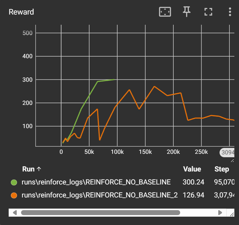
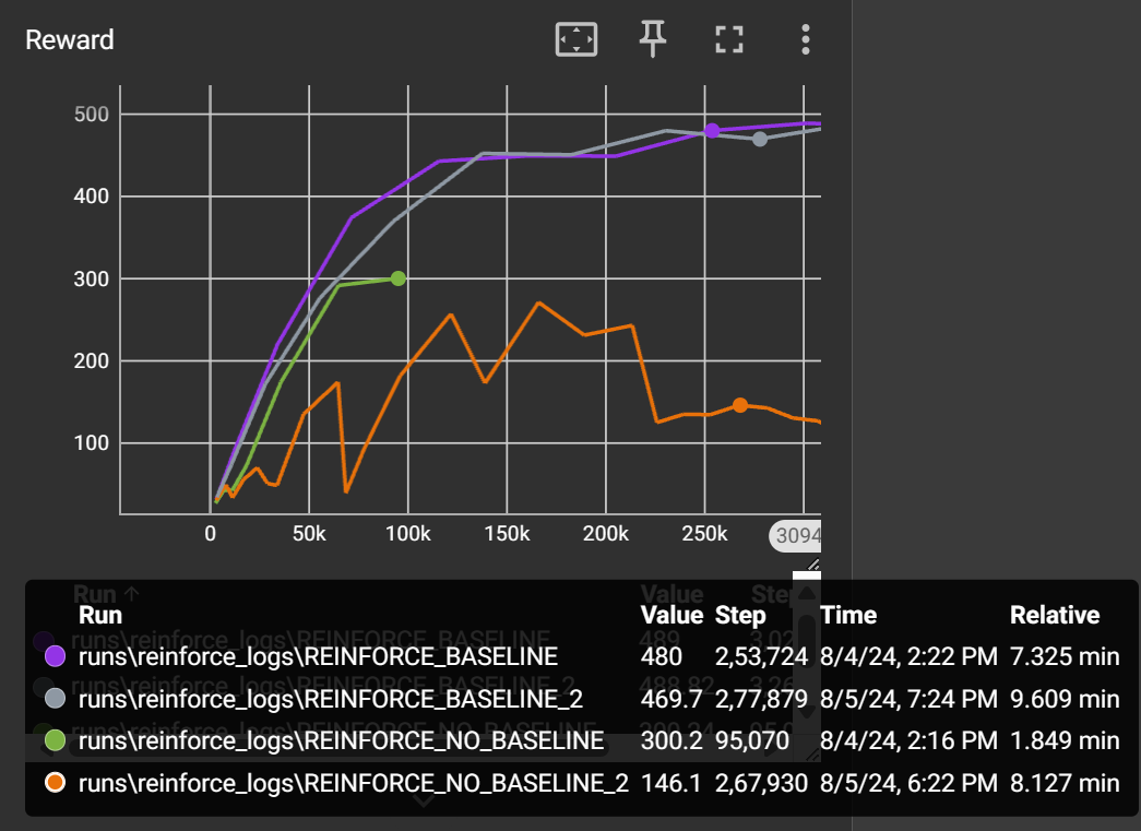
We can see that vanilla REINFORCE algorithm struggles to learn reliably. The learning is very unstable due to the high variance. The maximum reward in the CartPole environment is 500 and our agent is able to achieve 300. So there is scope for improvement. Now let’s see how baseline can help.

REINFORCE with Baseline (Value Policy Gradient - VPG)

Code Implementation: REINFORCE with Baseline

This code is almost similar. The only difference is that we have a value network and store the values during rollout. We use these values in the learn function to gain an advantage.

• Creating the Value Network

class ValueNet(nn.Module):
    def __init__(self, n_features, n_hidden):
        super(ValueNet, self).__init__()
        self.fc1 = nn.Linear(n_features, 256)
        self.fc2 = nn.Linear(256,128)
        self.fc3 = nn.Linear(128, 1)
  
    def forward(self, x) -> torch.Tensor:
        x = F.relu(self.fc1(x))
        x = F.relu(self.fc2(x))
        return self.fc3(x)

Then we just introduce the values in the agent class. I am not writing the whole code here as most of the other things are same.

    def __init__(self, env:gym.Env, lr, gamma, n_steps):
        
				self.value_net = ValueNet(env.observation_space.shape[0], 128).to(self.device)
        self.optimizer_value = AdamW(self.value_net.parameters(), lr=lr)
        
        #<SAME AS BEFORE>
        
    def rollout(self):
		   
			  #<SAME AS BEFORE>
        self.values = []

        
        while True:

	         #<SAME AS BEFORE>
           self.values.append(self.value_net(torch.from_numpy(state).float().to(self.device)))
           
           if terminated or truncated
           #<SAME AS BEFORE>
           
		def learn(self):
	        
        self.values = torch.cat(self.values)
        value_loss = F.mse_loss( self.values, returns)
				
				#<SAME AS BEFORE>
		
	      self.optimizer_value.zero_grad()
        value_loss.backward()
        torch.nn.utils.clip_grad_norm_(self.value_net.parameters(), float('inf'))
        self.optimizer_value.step()
        
        #<SAME AS BEFORE> 

Results

We can run this agent just like before.

The baseline version shows amazing improvements. The learning is stable, and the episodic reward grows consistently. So, if you ever have an episodic environment, REINFORCE with Baseline can be a viable choice.

Conclusion

In this part, we learned about the policy gradient method and wrote our first algorithm, REINFORCE. We saw that although this algorithm is powerful, it has some limitations,. Namely, it cannot work well with non-episodic tasks, and there is high variance. Thus, we must implement bootstrapping to reduce our dependence on complete episodic returns. We will look at this in the next part, where we will see our first actor critic method: Advantage Actor Critic (A2C). With that we will also see our first continuous action space implementation. Things are going to get exciting. Trust me!