Tabular Q Learning

16 Jul 2024

Reinforcement Learning is becoming the new trend. From controlling robots to optimizing logistics to tuning language models, reinforcement learning is the go-to strategy. However, newcomers to the field face a fragmented landscape and heavy reliance on implementation details. Even if you find a suitable RL algorithm from the many available, implementing it requires attention to fine details that aren’t part of the main RL algorithm, and getting these details right is challenging. While this is often problem-dependent, this series aims to show examples of implementation details across different RL problems and algorithms.

In this first edition, we explore the most basic form of Q-learning: Vanilla or Tabular Q-learning. You’ll see that even with the most basic algorithm, there are several tricks we can use to improve and adapt it to various problems.

This RL series is geared towards practitioners who already have basic knowledge of RL and have trained some basic RL agents. For this reason, I may not go into complete theory details and will mainly focus on finer implementation tricks. Nonetheless, let’s begin with some required basics. Also, in practice, one would use libraries like stable-baselines, but they are black boxes and do not provide a good understanding of how things work under the hood.

What is the agent’s objective in RL?

Every RL agent is trained for one simple objective: to maximize the total rewards accumulated. To do this, we need the agent to learn to take the most optimal decision in every state it can face. The equation below shows the total reward accumulated by the agent tarting at time step t.

Action-value function

The action-value function, often denoted as Q(s,a), is a fundamental concept in reinforcement learning. It represents the expected return (total accumulated reward) starting from a state s, taking an action a, and subsequently following a policy π. Formally, it can be expressed as:

The expectation can be resolved by running the agent in the environment for several iterations and updating the Q(s,a) for each state-action pair.

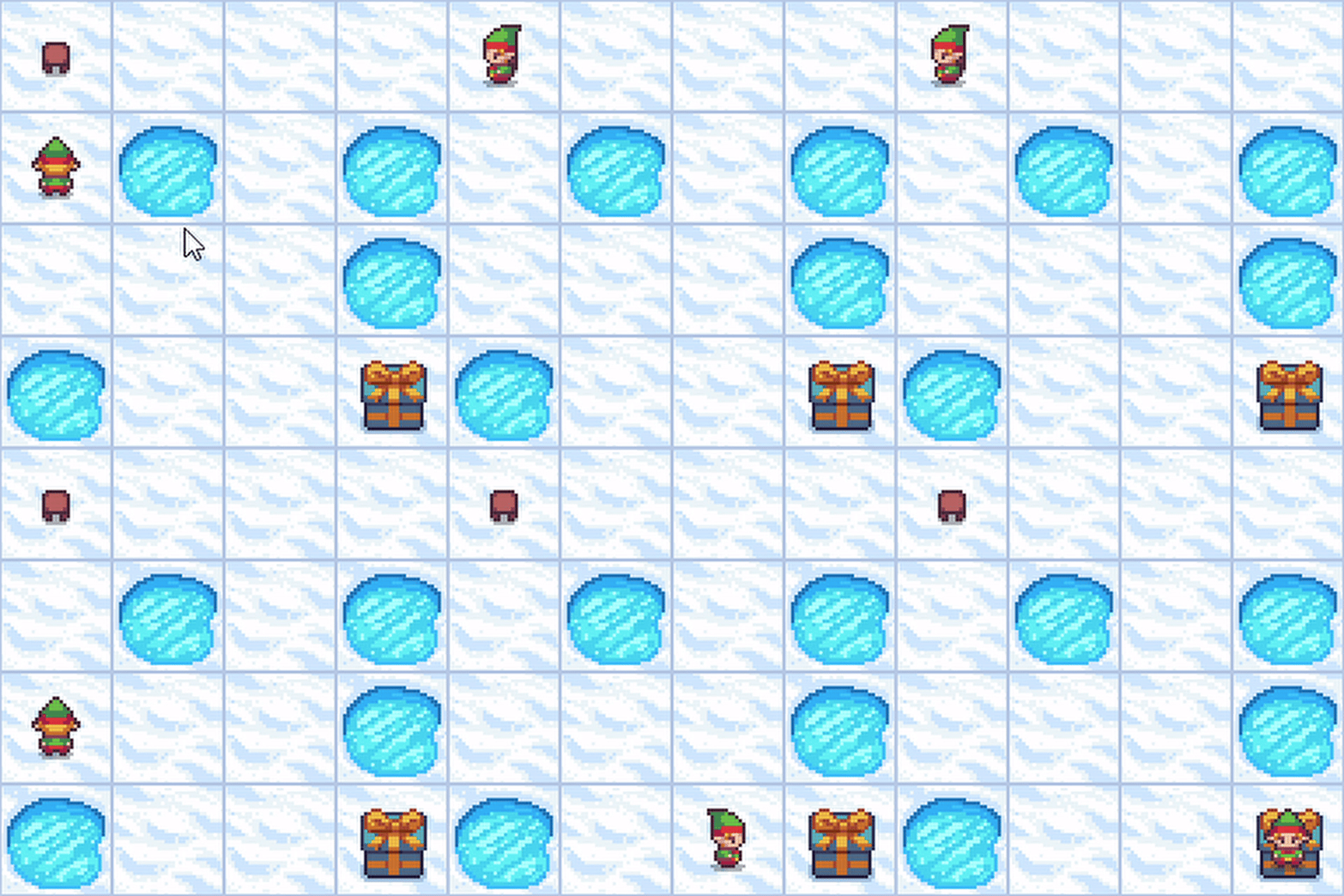
This is all the theory we need to implement our first Q-learning algorithm: Tabular Q-learning. Initially, we’ll use Tabular Q-Learning to solve the Frozen Lake Environment, ensuring our algorithm setup is correct. Following this, we will tackle the Pendulum Environment. This environment is chosen for several reasons: it has relatively few states and only one action. The states and actions are also continuous, meaning they can take any real value within specified limits. For Tabular Q-Learning, we require discrete states and actions. This scenario will demonstrate how we can modify the environment to fit our algorithm.

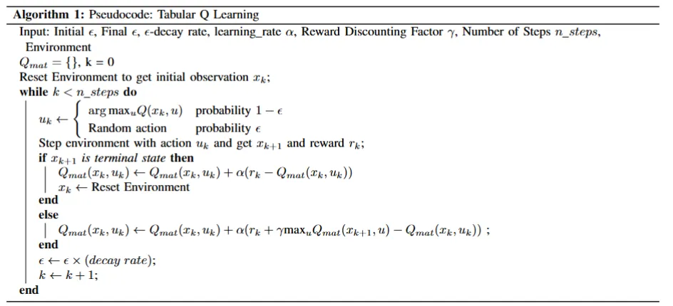
Pseudocode for Tabular Q Learning

1. Initialize Parameters: Set the initial values for all the parameters required for the algorithm. These include the exploration rate (ϵ), learning rate (α), reward discounting factor (γ), and the total number of steps the algorithm should run.
2. Initialize Q-matrix and Step Counter: The Q-matrix ($Qmat$) stores the Q-values for state-action pairs. Initially, it is empty. The step counter ($k$) keeps track of the number of steps executed.
3. Get first observation: The environment is reset to its initial state to start the learning process. The initial observation ($x_k$) is obtained from the environment.
4. Action Selection: At each step, the algorithm decides whether to explore or exploit. With probability 1−ϵ, it exploits by choosing the action that has the highest Q-value for the current state. With probability ϵ, it explores by choosing a random action.
5. Step Environment: The selected action is executed in the environment, which returns the new state ($x_{k+1}$) and the reward ($r_k$).
6. Check if Terminal State: If the new state is terminal (end of an episode), the Q-value for the state-action pair is updated using the reward received, and the environment is reset.
7. Non-Terminal State: If the new state is not terminal, the Q-value is updated considering the reward received and the maximum Q-value for the next state.
8. Decay ϵ: The exploration rate (ϵ) is decayed to balance exploration and exploitation over time.
9. Increment Step Counter: The step counter is incremented to proceed to the next step.
10. End While Loop: The process continues until the specified number of steps ($nsteps$) is reached.

Code Implementation for FrozenLake Environment

• First, let’s import the required dependencies. Here, we use the gym library, which was originally developed by OpenAI and has several environments for RL.

import gymnasium as gym
import numpy as np
from collections import defaultdict
from tqdm import tqdm
from copy import deepcopy
import matplotlib.pyplot as plt
from typing import Optional

• Next, we create a method for building the environment. For the FrozenLake environment, we build the environment as such without any modification, but in this method, we can wrap the environment in different modifications. We will see these modifications for the Pendulum Environment.

def get_env(
    env_name: str,
    render_mode="rgb_array",
) -> gym.Env:
    env = gym.make(env_name, render_mode=render_mode)

    return env

• We then define a custom argmax function to choose the action with the maximum q value. But if multiple actions have the same q value, this function chooses uniformly between the ties. The standard np.argmax function would just pick the first action and we don’t want that.

def argmax(a):
    # random argmax
    a = np.array(a)
    return np.random.choice(np.arange(len(a), dtype=int)[a == np.max(a)])

• Now we implement the main algorithm

def Qlearn(
    build_env,
    alpha=0.2,
    gamma=0.99,
    min_epsilon=0.1,
    nsteps=800000,
    Qmat=None,
    callback_freq=5000,
    callback=None,
):
    if Qmat is None:
        Qmat = defaultdict(float)

    episode_reward = 0
    mean_episodic_reward = 0
    n_episodes = 0

    epsilon = 1.0

    env: gym.Env = build_env()
    obs, info = env.reset()

    pbar = tqdm(range(nsteps), colour="green")
    for i in pbar:
        if np.random.rand() < epsilon:
            # Exploration: choose a random action
            action = env.action_space.sample()
        else:
            # Exploitation: choose the action with the highest Q-value
            action = argmax([Qmat[obs, i] for i in range(env.action_space.n)])

        next_obs, reward, terminated, truncated, info = env.step(action)
        episode_reward += reward

        if not terminated and not truncated:

            Q_next = max(
                Qmat[next_obs, action_next] for action_next in range(env.action_space.n)
            )  # Get the maximum Q-value for the next state

            # Update Q-value using Q-learning update rule
            Qmat[obs, action] += alpha * (reward + gamma * Q_next - Qmat[obs, action])

            obs = next_obs
        else:
            # Episode ends, update mean episodic reward and reset environment
            Qmat[obs, action] += alpha * (reward - Qmat[obs, action])
            n_episodes += 1
            mean_episodic_reward += (episode_reward - mean_episodic_reward) / n_episodes
            episode_reward = 0
            obs, info = env.reset()

        epsilon = max(min_epsilon, 0.99995 * epsilon)

        if i % callback_freq == 0:
            if callback is not None:
                # Execute callback function if provided
                callback(build_env, Qmat)
        pbar.set_description(
            f"Mean episodic reward: {mean_episodic_reward:.2f} | Epsilon: {epsilon:.2f} | Best reward: {best_reward:.2f}"
        )

    return Qbest

You can see here a few fine details:

• We initiate the $\epsilon$ at 1.0 and then decay it at every step by multiplying it with 0.99995 until it reaches some minimum epsilon. This decay rate becomes one of the hyperparameters.
• We are keeping track of the mean episodic reward.
• We have a callback function which we haven’t talked about yet. This is the test function that we define next. This is used for a couple of reasons. One needs to know how the greedy policy is performing because, in the end, we are going to just use the greedy policy. This is similar to a validation set that is used in Machine Learning. Another reason is to save the best-performing policy every time the test is performed. This is done to take into account the fact that RL algorithms face a phenomenon of catastrophic forgetting. This happens when the agent learns good policies, but then suddenly an update puts it on the wrong track, and it forgets what it has learned and then relearns. This is quite common with my RL algorithms and Q learning is one of them. That’s why we save the best policy so that if the agent is in a forgetting state at the end of the training, we can still retrieve the best policy. Here is the test code.

def test(build_env, Qmat, test_steps=1000):
    global Qbest, best_reward

    env: gym.Env = build_env()
    n_episodes = 0
    tot_rewards = 0

    obs, info = env.reset()
    for _ in range(test_steps):
        # Choose the action with the highest Q-value
        action = argmax([Qmat[obs, i] for i in range(env.action_space.n)])
        next_obs, reward, terminated, truncated, info = env.step(action)

        tot_rewards += reward
        obs = next_obs

        if terminated or truncated:
            n_episodes += 1
            obs, info = env.reset()

    if best_reward < tot_rewards / n_episodes:
        # Update the best reward and Q-best if a better reward is achieved
        best_reward = tot_rewards / n_episodes
        Qbest = deepcopy(Qmat)

    return tot_rewards / n_episodes

You can see that we check if the total reward during testing is better than the best rewards up to now, then update the best rewards and save the current *Qmatas Qbest.*

• Next, we just run the algorithm, by first initiating *Qbest* as None and best reward as -np.inf

Qbest = None
best_reward = -np.inf
build_env = lambda: get_env("FrozenLake-v1")

Qbest = Qlearn(build_env, alpha=0.1, callback=test, nsteps=100000)

• After training, we can just test the agent using this code

env = get_env("FrozenLake-v1", render_mode="human") # Slippery Frozen Lake is Default
obs, info = env.reset()
n_episodes = 3

for i in range(n_episodes):
    terminated = False
    truncated = False
    obs, info = env.reset()
    while not terminated and not truncated:
        action = argmax([Qbest[obs, i] for i in range(env.action_space.n)])
        obs, reward, terminated, truncated, info = env.step(action)

A new window opens, and we can see our little guy walking around. You will see that even though the ground is slippery the agent takes “safe” actions to both avoid the holes and still reach the goal.

Code Implementation for the Pendulum Environment

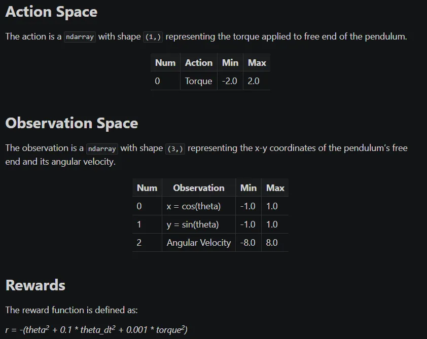
Alright, now that we know that our algorithm works for the Frozen Lake Environment, we are ready to switch to a slightly complex environment. For the Pendulum Environment, we need to make a few modifications because our algorithm supports only discrete observation and action space whereas the Pendulum environment has continuous observation and action space. So, we need to discretize the environmental spaces. We will be creating a wrapper for this. But first, let’s see what this environment contains.

So for the action space, we need to discretize the actions between -2 and 2. We can just choose a list of actions like [-2, -1.5, -1, -0.5, 0, 0.5, 1, 1.5, 2] , but this is manual and may not scale very well to other environments. Also, we need more actions that are smaller, because we need to have more fine control once the pendulum learns to swing up. Swinging up can be done easily using some large actions. For this, we can create a Gaussian kernel. A Gaussian kernel looks like this:

Here, A is the maximum value of the action. In our case, we have $\mu$ = 0. You can see that changing the sigma changes the way our actions are distributed. Thus $\sigma$ becomes one of the hyperparameters along with the number of actions available. Let’s define a function to create the Gaussian kernel.

def gaussian(x, mu, sigma, max_amp):
    return max_amp * np.exp(-0.5 * ((x - mu) / sigma)**2)

The above plot is created using this code:

x = np.linspace(-1, 1, 20)

# Compute the Gaussian kernel centered at 0 with standard deviation of 1
mu = 0
plt.plot(x, gaussian(x, mu, sigma=0.2, max_amp=2), label='Sigma = 0.2')
plt.plot(x, gaussian(x, mu, sigma=0.4, max_amp=2), label='Sigma = 0.4')
plt.plot(x, gaussian(x, mu, sigma=0.6, max_amp=2), label='Sigma = 0.6')

plt.xlabel('x')
plt.ylabel('Amplitude')
plt.title('1D Scaled Gaussian Kernel')
plt.legend()
plt.grid(True)
plt.show()

We are going to use $\sigma$ = 0.5 for the rest of the code. To discretize the state we use the formula,

Where nvec_s is the number of discrete states that we want to make. For this implementation, we are going to use [10, 10, 10], which means that the x value, y value, and the angular velocity of the pendulum are discretized to 10 values. For example, state corresponding to [0, 0, 0] will map to [-1, -1, -8], and state corresponding to [10, 10, 10] will map to [1, 1, 8]. Here is the code to do all this. We inherit the gym.Wrapper

class PendulumDiscreteStateAction(gym.Wrapper):

    def __init__(self, env: gym.Env, nvec_s: list[int], nvec_u: int, sigma: float):

        super(PendulumDiscreteStateAction, self).__init__(env)

        self.env = env
        self.nvec_s = nvec_s
        self.nvec_u = nvec_u

        # Check if the observation space is of type Box
        assert isinstance(
            env.observation_space, gym.spaces.Box
        ), "Error: observation space is not of type Box"

        # Check if the length of nvec_s matches the shape of the observation space
        assert (
            len(nvec_s) == env.observation_space.shape[0]
        ), "Error: nvec_s does not match the shape of the observation space"

        # Create a MultiDiscrete observation space and action space
        self.observation_space = gym.spaces.MultiDiscrete(nvec_s)
        self.action_space = gym.spaces.Discrete(nvec_u)

        # Define the possible actions
        
        kernel = gaussian(np.linspace(0, 1, 5), 0, sigma, 2)
        self.actions = (-kernel).tolist() + [0] + np.flip(kernel).tolist()
        # self.actions = [-2.0, -1.0, -0.5, -0.25, -0.15, 0.0, 0.15, 0.25, 0.5, 1.0, 2.0]

    def _discretize_observation(self, obs: np.ndarray[int | float]) -> np.ndarray[int]:

        # Discretize each dimension of the observation
        for i in range(len(obs)):
            obs[i] = int(
            (obs[i] - self.env.observation_space.low[i])
            / (
                self.env.observation_space.high[i]
                - self.env.observation_space.low[i]
            )
            * self.nvec_s[i]
            ) # equation: (x - min) / (max - min) * nvec
        return obs.astype(int)

    def step(self, action: int) -> tuple[np.ndarray[int], float, bool, dict]:

        action = self.actions[action]
        obs, reward, terminated, truncated, info = self.env.step([action])
        obs = self._discretize_observation(obs)
        return tuple(obs), reward, terminated, truncated, info

    def reset(self) -> tuple[np.ndarray[int], dict]:

        obs, info = self.env.reset()
        obs = self._discretize_observation(obs)
        return tuple(obs), info

Now we can modify our method to build the environment to include this wrapper.

def get_env(
    env_name: str,
    nvec_s: Optional[list[int]] = None,
    nvec_u: Optional[int] =None,
    time_limit: Optional[int] = None,
    sigma: Optional[float] =  None,
    render_mode="rgb_array",
) -> gym.Env:
    env = gym.make(env_name, render_mode=render_mode)

    if nvec_s is not None and nvec_u is not None:
        env = PendulumDiscreteStateAction(env, nvec_s, nvec_u, sigma=sigma)

    if time_limit is not None:
        env = gym.wrappers.TimeLimit(env, max_episode_steps=time_limit)

    return env

We can also provide a different time limit to end the episode within a certain number of steps. Now, we can just call the Qlearn method again to train the agent on the new environment.

build_env = lambda: get_env("Pendulum-v1", [10, 10, 10], 11, 200, sigma = 0.5)
Qlearn(build_env, alpha=0.2, callback=test, nsteps=1000000)

As you can see, the agent learns to swing up pretty well, but keeping it centered on the top is quite hard. This shows that Tabular Q Learning is not the best method for complex environments. This is because discretizing to just 10 states yields 10 x 10 x 10 observation space. And this increases rapidly with more states and more discretization. Thus we need a better method. In the next part, we will look into Deep Q Learning, which uses a neural network to map the states to the Q values.

Git Repo: https://github.com/akshayballal95/rl-blog-series/tree/tabular

---